|
M 10/1/07
|
HW due: Read pp. 107-117; write #3.8. The step-by-step
button-pushing instructions are provided in your textbook. I recommend that you
practice several times until you can quickly make a scatterplot to show any
2-variable relationship, since we will be doing a lot of that this year.
|
|
|
T 10/2/07
|
HW due:
1. Gather the height (in inches) and shoe size of 10 male friends. Record your
data in a handwritten table of three columns, labeled NAME, HEIGHT, and
SSIZE. Enter your data in lists named HEIGHT and SSIZE (similar to
yesterday’s exercise). As we did in class yesterday, press STAT CALC 8 but
then enter LHEIGHT,LSSIZE,Y1
and press ENTER. Note: You do not
type the list names; you choose them from the 2nd LIST menu. The Y1
function keystrokes, as you know, are VARS Y-Vars Function Y1. You
may share some data with
classmates, but your list of 10 students should be uniquely your own.
The command is therefore going to look like this on your screen:
LinReg(a+bx) LHEIGHT,LSSIZE,Y1
When you press ENTER, the calculator will display the regression coefficients
(intercept and slope). Use 2nd STAT PLOT to define a scatterplot that uses
HEIGHT as the Xlist and SSIZE as the Ylist. When you press ZOOM 9, you should
see a scatterplot with the regression line overlaid.
2. Transcribe your scatterplot and regression overlay onto paper. (Neatly,
please. It does not have to be perfect, but take a few minutes to make it
look decent.)
3. What linear correlation coefficient did you find? Write r = ______ . Remember, your r value is not displayed at the time
of performing the regression unless you have set the DiagnosticOn feature as
we did in class yesterday. This command is found under 2nd Catalog.
|
|
|
W 10/3/07
|
HW due:
1. Prepare for your weekly “Quick Study” quiz.
2. Read pp. 117-135, omitting the exercises. However, read all of the examples
with a calculator and a notebook by your side. The total amount of reading is
therefore about 9 pages, certainly reasonable. Remember that reading notes
are required, as always.
3. Write #3.14 (using Table 3.3 on p. 126), 3.24.
|
|
|
Th 10/4/07
|
HW due: Make sure you are caught up on all previously
assigned problems, and write #3.16.
|
|
|
F 10/5/07
|
Faculty
professional day (no school).
|
|
|
M 10/8/07
|
Holiday
(no school).
|
|
|
T 10/9/07
|
HW due: Write #3.50 on pp. 165-166 before and/or after
carefully reading pp. 137-142. Pay special attention in your reading notes to
Example 3.10 on pp. 141-142. Note the following crucial sentences excerpted
from p. 142:
1. “When you write the equation, don’t forget the hat symbol over the y; this means predicted value.”
2. “The slope b = .1890 in this
example says that, on the average, each additional degree-day predicts
consumption of 0.1890 more hundreds of cubic feet of natural gas per day.”
3. “The intercept of the regression
line is the value of  when x = 0. Although we need the value of
the intercept to draw the line, it is statistically meaningful only when x can actually take values close to
zero.” when x = 0. Although we need the value of
the intercept to draw the line, it is statistically meaningful only when x can actually take values close to
zero.”
Of these, which are all important, #2 is the most important of all. In fact,
every AP exam and practice AP exam I have ever seen contains at least one
question asking for the interpretation of the linear regression slope in
context.
For learning purposes, we should reword the quoted excerpt in #2 above,
putting it into a more general context. To this end, assume that the slope of
the LSRL is 123.456. Let x
represent the number of widgets, and let y
represent the number of wombats. (These are made-up names and numbers for
illustrative purposes only.)
Here is the reworded interpretation of the slope:
“A slope of b = 123.456 means that
each additional widget predicts, in the
model, an increase of 123.456 wombats on average.”
If the slope were –123.456, we would say, “A slope of b = –123.456 means that each additional widget predicts, in the model, a decrease of 123.456
wombats on average.”
Let’s try another one to make sure that you understand the pattern. If b = 4.3, if x refers to florms, and if y
refers to glorms, then the answer to the question about interpreting the LSRL
slope would be as follows:
“A slope of b = 4.3 means that each
additional florm predicts, in the
model, an increase of 4.3 glorms on average.”
Additional hints for #3.50: You do
not actually have to do the reading in order to solve #3.50. Our in-class
exercise, in which we empirically found that the, ahem, LSRL for dating is
approximately

gave us an example of finding the LSRL slope and intercept by using STAT CALC
8 L1,L2,Y1 . . . which is exactly what you
will be doing in #3.50.
(a) You should be able to answer this without punching a single button.
(b) Use your calculator. Put boat registrations in L1 and manatee
deaths in L2. (Note: Year is a possible lurking variable, but we
will not do anything with the years for now.) Use 2nd STATPLOT to make the
scatterplot, and transcribe it (roughly) to your paper.
(c) Answer the first question based on the appearance of the scatterplot. To
answer the second question, punch 2nd QUIT followed by STAT CALC 8 L1,L2,Y1
so that you can get the r2
value.
Note: If you were absent on the day
that we set DiagnosticOn, or if your calculator has been rebooted since then,
you must perform a Google search for the word DiagnosticOn as a single word.
Either of the first two hits will give you the instructions you need.
<sarcasm>Of course, you could try reading your calculator manual, but I
seldom recommend anything as drastic as that.</sarcasm>
(d) Your calculator will do the drawing for you when you press ZOOM 9. Simply
transcribe the sketch onto your homework paper. The parenthetical instruction
“Use Minitab’s work” means that you can check the predicted number of manatee
deaths by pressing TRACE [down arrow] 700 ENTER, but to show your work, you
need to write the following (and you may copy my work if you wish):

The model predicts 43.9 manatee deaths per year if powerboat
registrations are frozen at 700,000.
[This value differs slightly from the TRACE value because of rounding errors
in the a and b statistics.]
(e) Simply circle the data point (716, 35) on your scatterplot. There is
nothing bizarre or special about the year 1993 that would cause us to remove
this data point.
(f) This question is a throwback to the earlier material on normal distributions.
I agree that the question appears complicated, but it is really only asking
how surprising a residual would be if it came from a normal distribution and
had a z score of –2.08. How often
does this happen through chance alone?
|
|
|
W 10/10/07
|
Cumulative Test (100 pts.), focusing
on pp. 83-142. Although the test
will focus on pp. 83-142, and you can probably pass it simply by studying
those pages, the truth is that you cannot forget the basics that we learned earlier:
What is a statistic? What is a parameter? What is a z score? What is a percentile? What score on a Ms. Denizé test
with mean 73 and standard deviation 5 would be at the 90th percentile? What
percentage of students are between 72 and 75 inches tall if the mean is 71
and the standard deviation is 3? What is meant by response bias, or bias in
general? How do we go about proving cause and effect? How do we determine
outliers? How do we compute PPV? What is the 5-number summary? What is the
notation for sample size? sample standard deviation? population variance?
interquartile range?
|
|
|
Th 10/11/07
|
No
additional written HW due. However, there will probably be a quiz on the
“Quick Study.” If you have additional time, please read pp. 144-788. (Just kidding.
We will ultimately read all the way to p. 788, but not tonight. Just read as
many pages as you feel comfortable reading.)
|
|
|
F 10/12/07
|
HW due: Read pp. 144-160 (especially the summary on p.
160), plus the LSRL Top Ten;
write #3.40.
|
|
|
M 10/15/07
|
HW due: Print out last week’s
test and re-do the entire thing (even the parts you are fairly sure you
did well on). Note that sketches of normal curves are required for #21-23,
unlike on test day, when I allowed you to write answers only.
Try to do this exercise “closed book, closed notes,” but of course you may
need to open your book to consult the z
table. Using notes or textbook is permitted, but please, please, push
yourself as hard as you can before you break down and use your notes or
textbook. You’ll learn more that way, even though it may take more time and
will definitely involve more frustration.
You may work with friends if you wish, as long as you document the
collaboration, but each student must have a test in his own handwriting. Here
is an example of how you might document the collaboration:
“I, Joseph W. Bulldog, certify that the work presented here is my own, except
for #7, which I obtained from Willie, and #21-23, which I didn’t understand
at all until Lawton explained them to me. I provided answers for #8 and #9 to
Alex, and Alex and Kevin helped me understand #19, although my original
answer for #19 was fairly close.”
Scoring: If your work is well done, I may use it to adjust your entire test
score in a favorable direction. If your work is slapdash, incomplete, or
obviously copied (as opposed to collaborated), I will treat it with no
special deference. How can I tell if work is copied? Well, remember that I
have been doing this for many years and have a host of tricks up my sleeve. I
think I told you how I was able to break up a HappyCal copying ring last
year.
|
|
|
T 10/16/07
|
HW due: Write #3.51, 3.52.
In class: Go over #3.52 and explain why the answers are 6, 2, 5, 8, 3, 7, 4,
1.
Then go over #3.51 and explain why the association is negative (not “inverse” as some people said on the most recent
test). The regression line is  , where x = year
in YYYY format and , where x = year
in YYYY format and  = predicted mile record in seconds. = predicted mile record in seconds.
Is there an apparent trend? Yes, a
strong negative linear association.
Calculate the correlation. r =
–0.983
Comment on the suitability of the LSRL as a model for the data. Scatterplot suggests suitability. However,
the residual plot shows some waviness, suggesting that record improvements
ebb and flow.
Interpret the correlation. The r value
of –0.983 shows strong negative linear association. The r2 value
of 0.9665 shows that almost 97% of the variation in the mile record can be
explained or predicted by variation in the year.
Are there any regression outliers? Yes,
the data points for 1868, 1882, and 1884 appear to be outliers.
Influential observations? No.
On average, how many seconds are lopped off this record each year? About 36 hundredths of a second (as given
by the LSRL slope).
Would you feel comfortable predicting the world record . . . in the year
2000? Maybe. The LSRL predicts 3:41.53
for the year 1999, which matches fairly well against the actual figure of
3:43.13. However, one thing your textbook could not predict is that
high-level track meets are now almost all conducted at metric distances, and
there has been no progress on lowering the mile record since 1999. This
example illustrates another (non-mathematical) danger of extrapolation.
. . . in 2005? No, that would clearly
be extrapolating too far. That would give a time of 3:39.35, which is
seemingly impossible with today’s equipment and training methods.
|
|
|
W 10/17/07
|
“Quick Study” Quiz (10 pts.) at beginning of class. If you miss it, you miss it.
HW due: Read pp. 164-165, 176-177,
179-188. Then perform the steps below. Steps 2 and 3 involve written work.
1. Execute Example 4.1 (pp. 179-182) step by step on your calculator and make
all lists and scatterplots exactly as shown in the text. There is no written
work to do here, but I will probably check to make sure that your lists and
scatterplots are complete. If you have trouble, I expect you to work with a
friend or use the Web to find calculator keystroke techniques. (You may even
have a calculator manual you could consult.)
2. On p. 184, key the YEAR data into list L4 and the MBBL data
into list L5. Make a scatterplot in Plot 2 (so that your earlier
work from Example 4.1 is not lost) and transcribe the result onto your paper.
3. On p. 185, perform algebraic simplification on the third equation (the  equation in the
middle of the page) to put it in the form equation in the
middle of the page) to put it in the form  where a and b are constants. Show your work. where a and b are constants. Show your work.
4. Finally, perform an exponential regression (STAT CALC ExpReg L4,L5,Y2)
as you learned in Precal. Verify that your calculator gives the same result
as the one you obtained in step 3.
|
|
|
Th 10/18/07
|
HW due: Read all 5 pages of this article from the
current issue of New York and the companion article as well (1
additional page). Be prepared to discuss both articles in depth.
|
|
|
F 10/19/07
|
Form
VI retreat (no class).
|
|
|
M 10/22/07
|
HW due (for many): Group exploratory
data analysis project. This is due
by the end of the week for everyone. Please shoot for Wednesday or Thursday,
so that there is not a last-minute crunch. I am happy to offer constructive
criticism on draft versions as a way of maximizing each group’s chances of
earning an A.
General instructions regarding your report:
- Begin by describing your research question, an
overview of your findings, and your methodology. You may call the
overview an “executive summary” if you like to use buzzwords from the
business world.
- In the main body of your report, analyze your
findings by providing visual depictions of the data, accompanied by
statistics (5-number summary and the like). If there are any outliers,
gaps, or unusual findings, you would want to call attention to them and
explain them if possible. Similarly, a lack of unusual findings is also
worth noting.
- After your analysis, give a summary of your
report. If there is any deeper meaning, you would want to say what it
is. (There may not be any.) List any lessons learned as well as things
you might do differently if you were doing the project afresh. If
possible, suggest some areas for future research of related questions.
- Important: Include, as an appendix, a
spreadsheet table of your raw data, one row per data point.
- After the appendix, the group leader should
include a statement (1-2 paragraphs) recommending the point split among
group members and documenting, in some detail, the reasons for that
point split. Describe what parts of the work were done by each person.
If anyone was unreliable or missed meetings, mention that unless the
person made amends that everyone in the group found acceptable. If the
group leader’s statement is missing, his score will be reduced by 10
points.
- Since we are not running an experiment, your
analysis does not need to be as extensive as it will be later in the
course. The total length of your project report will probably be 5 pages
or fewer. Some groups may need only 2 to 3 pages to have a good project.
Try to be concise, using words to emphasize (but not restate) things
that the charts already show. For example, if you had a scatterplot
showing a positive linear association, here are two approaches:
Example
#1 (weak):
The
scatterplot (Fig. 1) shows a positive linear association between the
explanatory and response variables. The least-squares regression line slopes
steadily upward with a slope of 1.5 and crosses the y-axis at a y-intercept
of 4.3. The value of the linear correlation coefficient, r, is approximately equal to 0.848.
[This
is wordy and contains nothing that the graph with a labeled LSRL does not
already say. It is also excruciatingly boring to read. Have pity on your poor
teacher, who must grade your project.]
Example
#2 (much better):
Although
the positive linear association shown in Fig. 1 is strong (r = 0.848), there are two outliers
shown in red. Both of those data points were for days when more than 50
students were absent for field trips or sporting events. Since the remaining
students who attended lunch were likely to have been quieter than average,
they did not display the pattern seen on the other days, even when size
differences between refectory crowds are taken into account.
|
|
|
T 10/23/07
|
HW due: Read pp. 190-195 and summary on p. 197; write #4.4,
4.7. To help you, some work related to yesterday’s height-weight example is
shown below.
List of xi (explanatory)
= HT = {72, 69, 70, 71, 75, 72, 71, 71.5, 71, 73, 71, 75, 72}
List of yi (response) =
WT = {158, 156, 170, 150, 200, 145, 165, 162, 175, 195, 160, 185, 175}
LSRL: 
The LSRL fit is good, since r =
0.675 (absolute value close to 1) and the residual plot is quite random.
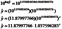
Next, try an exponential fit. That means that we have to compute a LSRL
between the x values and the log of
the y values. [The calculator steps
for this are log(L2) STO L3 ENTER STAT CALC 8 L1,L3,Y1
ENTER.]
LSRL relating x values to the log
of y: 
To “perform the inverse transformation” (to use your book’s terminology), we
perform algebra on that equation, beginning by taking 10 to the power of each
side:

As a check on your work, punch STAT CALC 0 L1,L2,Y1
and observe that the exponential regression produced by your calculator matches
(with a slight roundoff error) the answer shown above in the final line.
The exponential fit is curved. Even though its residual plot is not
noticeably better than the residual fit for the LSRL, the fact that the
exponential fit is curved would help it do better for forward or backward
extrapolation. After all, we know (don’t we?) that people’s weights do not
grow as a linear function of height.
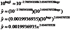
A still better fit is the power regression fit. Remember, the hallmark of a
power relationship is that the log of y
is a linear function of the log of x.
(This is different from exponential, where the log of y is a linear function of “just plain” x.)
LSRL relating log x values to the
log of y: 
As above, we “perform the inverse transformation” by taking 10 to the power
of each side:

As a check on your work, punch STAT CALC A L1,L2,Y1
and observe that the power regression produced by your calculator matches the
answer shown on the last line above. The r
value for the log x to log y linear fit is somewhat lower than
the r value for the original LSRL,
as well as for the exponential fit (x
to log y), but the power regression
model is desirable. Not only is it curved, but since the power regression
function passes through the origin, it allows much better forward and
backward extrapolation. Of course, extrapolating all the way back to the
origin (0 pounds predicted for a height of 0 inches) would be ridiculous, but
that still makes more sense than what either of the other two regression
equations would produce.
|
|
|
W 10/24/07
|
Test (100 pts.) on all recent material, including
linear and nonlinear regression.
Terminology (IQR, population and sample variance, z-scores, etc.) will also be tested, as always. The formulas
listed below will be provided for you on a formula sheet. Although you do not
have to memorize them, you must be thoroughly familiar with all but 3 of
them. Having them listed will do you no good unless you know what each letter
means and how the formulas would be applied.


 [pooled estimate of
sample proportion; not used] [pooled estimate of
sample proportion; not used]

 [true, but not used;
use your STAT CALC 8 instead] [true, but not used;
use your STAT CALC 8 instead]


 [standard error of
the LSRL slope; not used] [standard error of
the LSRL slope; not used]
Study help: Here are the remaining
answers to #4.4 from yesterday’s HW assignment.
(e) My answer is different from the book’s answer key, which I think contains
an error. The linear regression equation fitting log y to log x is

Therefore, 


This matches the equation that the power regression (STAT CALC A) produces.
To answer the remaining two questions, we plug in 70 and 84, respectively, to
get


|
|
|
Th 10/25/07
|
No
additional HW due today.
|
|
|
F 10/26/07
|
HW due: Finish your group project report and turn it in by
class time. In an emergency situation, I may allow an extension until 3:00
p.m., but only if the extension is requested in a timely fashion. (Think
about it: If you request the extension, breathless, at 10:45 a.m., you are
admitting a failure to plan ahead, since surely you were aware earlier that
you needed an extension.)
If you have already submitted your project report (congratulations to Kevin,
Willie, Will, and Bobby!), then you have no HW.
|
|
|
M 10/29/07
|
First
day of second quarter (no additional HW due). If you wish to work ahead,
textbook reading is always safe, since we will cover the entire book through
p. 788.
|
|
|
T 10/30/07
|
HW due: Read pp. 206-217. Since virtually all of this has
already been covered in class, reading notes are optional this time.
|
|
|
W 10/31/07
|
HW due: Prepare for your weekly quiz, and submit a group proposal
for the second project (experiment). At this point, you do not need much in
the way of detail. A few concepts, with simply a research question and a
sketchy description of your experimental design for each, will suffice.
|
|


