|
Th 3/1/07
|
HW due: Read pp. 567-574, and re-do the entire test from yesterday, even the problems you think
you answered correctly. This assignment is required even if you were absent
yesterday.
You may work with other students, but you may not copy their writing. What
you write must be your own. You must show work for #7(a), even though work
was optional during yesterday’s test.
|
|
|
F 3/2/07
|
HW due: For each of the following, write (a) a null and
alternative hypothesis, (b) an example of Type I error, and (c) an example of
Type II error. The first one has been done for you as an example.
1. Car alarm.
(a) H0: Situation is
normal (no break-in is in progress).
Ha:
A break-in is in progress.
(b) False alarm.
(c) Burglar breaks in, but the alarm does not go off.
2. American court system: A person is indicted on a criminal charge and is tried
by a jury.
3. TB (tuberculosis) test.
4. Lie detector test for screening potential CIA employees.
5. PSAT/NMSQT test to identify exceptionally gifted students to be National
Merit Scholars.
6. Mr. Hansen performs a random homework audit to ensure that students are
rating themselves correctly.
7. A government chooses to investigate any taxpayer whose deductions exceed
AGI (adjusted gross income) by more than a factor of k, for some positive value k
to be chosen each year. The taxing authority recognizes that it may waste
some time pursuing innocent people but reasons that most of the people whose
deductions are more than k times
their AGI are guilty of tax fraud.
8. A spam filter automatically deletes any incoming e-mail message containing
more than a certain number of key words (Viagra, Nigeria, Cialis, etc.),
because these words are typically found in many spam messages.
9. A computer remains locked up and inaccessible until a user with a matching
fingerprint (or, at least, a fingerprint that is close enough to be
interpreted as a match) uses the fingerprint scanning device. At that point,
the computer unlocks itself and provides access to the user.
|
|
|
M 3/5/07
|
Double
Quiz on Type I and Type II error.
You will not need to calculate the probabilities today. All you will need to
be able to do is to explain what Type I and Type II error are, write null and
alternative hypotheses, and give examples of what would constitute Type I and
Type II error in various situations. In other words, you must be able to do
the types of things we discussed Friday.
There is no additional written work due today.
|
|
|
T 3/6/07
|
Oops! No additional HW since it was not posted in
time. However, if you have a few minutes, please reread the material on the
LOLN (pp. 389-394 and 492-494) so that we can discuss it intelligently.
Reading notes are optional this time.
|
|
|
W 3/7/07
|
Quest (70
pts.) on all recent material. The alternate test on Chapter 9 and Beginning of
Chapter 10 furnishes a good review, except that you also need to know
Type I error, Type II error, and power, where “power” is defined as 1 – P(Type II error). You will not be
required to perform numeric calculations involving Type II error and power,
but you need to know the concepts we discussed.
We covered problems #1-5 in class and/or on the previous test. Answers to the remaining problems are available
now to assist you as you study.
|
|
|
Th 3/8/07
|
HW due: Reread pp. 389-394 and 492-494, and make sure you
have reading notes on the specific topic of LOLN if you did not prepare some
the first time. Then for your written assignment, do the following:
Let H0: m = 6 and Ha:
m < 6 be our
hypotheses, and let s = 4.8. Let
the sample size be n = 25. We will
use a = 0.05 for now.
Remember, a is a “cutoff value”
for P, .i.e., the value of P below which we will reject H0.
1. What test should we use (2-sample t,
1-prop. z, chi-square, etc.)?
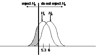
2. Draw a sketch to estimate the power of the test against the alternative m = 5.3. In other words, how effective is the test at
avoiding Type II error if the true value of m happens to be 5.3? Your sketch should include two
sampling distributions (null and alternative), as well as a clear vertical line
that separates the “reject” and “do not reject” regions.
3. Draw a sketch to show how your answer to #2 changes if s is decreased, but everything else
stays the same.
4. Draw a sketch to show how your answer to #2 changes if s is increased, but everything else
stays the same.
5. Draw a sketch to show how your answer to #2 changes if the alternative of
interest is farther to the left of the H0
value (say, m = 3.1 instead of m = 5.3), but everything else stays the same.
6. Draw a sketch to show how your answer to #2 changes if the a level of the test is adjusted from .05 (a typical
value) to .01 (a stringent value designed to reduce the probability of Type I
error), but everything else stays the same.
|
|
|
F 3/9/07
|
No additional HW due, but that doesn’t mean you’re
off the hook. Please re-do your HW that was due yesterday so that it is of
good quality. (Nobody attained that level yesterday.)
Optional Bonus (up to 3 pts.): For
the problem we were working on in class (namely, the power of a t test for speeding with H0: m = 75, Ha:
m > 75, s = 5, a = .05), plot the test’s power against the 80-mph
alternative as a function of n. We
already know that for n = 9, the
power is approximately 85%, and for n
= 10,000, the power is essentially 100%.
|
|
|
M 3/12/07
|
Form VI Career Day—class canceled for everyone.
|
|
|
T 3/13/07
|
Quiz (10
pts.) on the formula sheet. You
will be given a blank AP formula sheet and will be asked to mark each formula
on the first two pages as (1) irrelevant or calculator-handled, (2) useful,
or (3) in need of a rewrite. In the event of a rewrite, you must furnish the
rewritten version. On the t table,
you must identify the df = ¥ row as signifying z*.
Finally, you will be asked to identify some or all of the formulas on the
third page, going in either direction. For example, if I point to the second
formula, you would indicate that it is used for both the 1-prop. z test ( ) and the 1-prop z
confidence interval ( ) and the 1-prop z
confidence interval ( ). ).
If I ask which formula is used for a 2-prop. z test, you would say, “the last one in the last box, usually.”
If I ask what the second formula in the “difference of sample means” box is
good for, you would say, “nothing.” STAT TESTS 1, 3, 7, and 9 are not used.
You can memorize all of the third page by writing the following codes keyed
to the TI-83 in the right margin:
2,8
5,A
4,0
X (not used)
B
6 (usually)
C or CSDELUXE
HW due (10 points): Read pp.
576-580 and redo the assignment that was due Thursday 3/8, even if you
already turned it in. There were no acceptable papers, and everyone should
redo the assignment on a fresh sheet of paper. Two students came close, but
one paper was sloppy and the other did not properly identify the change that
had occurred in each case. (You must say “power increases” or “power
decreases.” You cannot assume that the reader can tell what has happened,
especially since most of you shaded the Type II error instead of the power or
shaded something completely irrelevant, such as the area underneath the
overlap of the two curves.) This homework was scored twice in the third
quarter, costing many people 8 points. Notice that 8 points is the same as
the difference between a 91 and an 83 on a test, which most students would
view as significant, but for some reason many students seem happy to throw
away 8 homework points. This time the assignment will be scored as a quiz in
the hope that you will work hard on it.
Example of what I expect for problem #2 and a problem that was not posed
originally are below. You may copy my work for #2, because it is difficult.
All of the other problems, except for #6, can be done qualitatively. You
should come up with a numeric answer for #6.
2. Sketch:

To find the power, we begin by computing s.e. = s/Ön = 4.8/Ö25 = 0.96. Second, note that we can estimate our power fairly closely
by using the z distribution. The
cutoff value for significance is 4.42094 [calculator keystrokes: invNorm(.05,6,.96)].
Finally, power equals the area of the alternative distribution that lies in
the “reject” zone, which is .180 [calculator keystrokes:
normalcdf(-99999,4.42094,5.3,.96)].
Remember that you cannot show calculator keystrokes on your writeup unless
they are Xed out.
(Optional.) Doing #2 with t
distributions, which is more correct, is unfortunately more difficult. Since
your calculator does not accept mean and s.d. (s.e.) of the sampling
distribution in its tcdf function, you must use the formula t = (obs. – hyp.)/s.e. to convert back
and forth between t units and
“observed units.” I do not expect you to be able to do this reliably, but I
do expect you to read the steps below and figure out what is going on. The
mnemonic is “TOOTAR.”
(t0)
Find the cutoff t score for the H0 distribution. From Table
C, this is –1.711. (We use the df = 24 row, since df = n – 1 for a 1-sample t
test, and the reason for the minus sign is that we are using a left tail.)
(o)
Find the “observed units” for that t
score. By the equation t = (obs. –
hyp.)/s.e., we have –1.711 = (obs. – 6)/.96, which we solve (using Algebra I
skills) to get 4.35744.
(ta)
Rewrite 4.35744 as a t score in the
alternative distribution. Again using our equation t = (obs. – hyp.)/s.e., we have t = (4.35744 – 5.3)/.96 = –.9818333.
(rejection
area) Find the power (i.e., the area of the Ha distribution that lies in the “reject” zone) by
using tcdf and part (c). [Calculator keystrokes are
tcdf(–99999,–.9818333,24), but remember that you cannot show those unless you
X them out.] The answer, .168, is reasonable based on the sketch. This
answer also compares favorably with the .180 that we quickly obtained above
by using z distributions (ZOOZAR?).
The z method is fairly easy, since
your calculator does most of the work, but TOOTAR may be too hard for some
students.
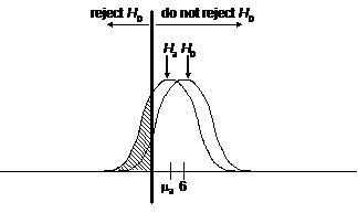
7. Draw a sketch to show how power changes if we allow a greater level of
Type I error, and if we shift the alternative hypothesis slightly upward, but
if everything else stays the same.

We know that there is usually a tradeoff between Type I and Type II error:
allowing Type I probability to increase will allow Type II error to decrease,
thus increasing power. (One exception to this tradeoff rule is an increase in
n, which will reduce both the
probability of Type I error and the probability of Type II error.) In this
problem, however, ma has
shifted to the right. The diagram, as drawn, shows that power (shaded) has
stayed exactly the same. We may summarize this concept by saying that if the
alternative of interest is moved closer to the null hypothesis, then power
will decrease unless we accept a higher probability of Type I error, in which
case we may be able to keep power the same.
|
|
|
W 3/14/07
|
HW due: Read pp. 587-608 (see instructions below) and this
article from Monday’s Post;
write #11.18.
Note: From now until the end of the
year, I do not expect you to read all the assigned pages from the textbook
thoroughly. Instead, I will identify the most important passages and will ask
that you skim the entire block of pages, with special attention paid to the
highlighted areas. For today you must read pp. 594-596 and 605-606
thoroughly; everything else on pp. 587-608 is worthwhile but may be skimmed.
Do not skip over the examples! When I say pp. 594-596, I mean all parts of
all three pages. The passage for pp. 605-606 starts after exercise #11.14 on
p. 605.
|
|
|
Th 3/15/07
|
HW due: Skim pp. 610-656 to become familiar with the
topics. As it turns out, the only pages you need to read carefully are pp.
629-631. Then write #11.69.
Note: Use 90% confidence intervals.
(That means that your answers will not match the answers given in the back of
the book, but you can temporarily use 95% intervals to see if you can match
the book’s answers, as a way to make sure that you are punching the buttons
correctly.) The answers given in the back of your book are not in an
acceptable format because they do not describe, in words, the differences
between the runners. Your answers should begin with the following words:
“We are 90% confident that the difference of mean abdominal body fat . . .”
“We are 90% confident that the difference of mean thigh body fat . . .”
You need not show all of your work, since the calculation of df is
horrendous. (Glance at the formula on p. 633, but be careful not to look at
it too long! It may scar you for life.) However, you should show the
calculation of s.e. By using your calculator’s answer and working backwards,
you can deduce what the t* value
must be.
Here is what I mean. For the 95% C.I. for abdominal body fat measurement, we
know that the answer is –15.4 to –11.6, i.e., –13.5 ± 1.884. Therefore, m.o.e. = 1.884. We show our work
as
 , ,
where the t* value of 1.983 is
actually “reverse engineered” from what we know it has to be to get the
answer to work out correctly. You can’t get 1.983 from your t table, because finding the df is a
horrifying task that is best left to your calculator. Besides, even if you
knew the df (which is 103.6), you’d still have to estimate, since there is no
row for 103.6 in the table. All of these calculations are easy with a
graphing calculator or a computer, of course, which is why we use the
technology. Please observe, however, that the t* value of 1.983 is certainly reasonable, since the table tells
us that t* for a 95% C.I. is 1.984
if df = 100.
The main reason to show your work for m.o.e. is to show that you know how to
find the correct s.e. formula on the third page of your formula sheet. You
need practice doing this, which is why I am making you do it.
One final note: C.I. answers for differences of means are much easier to
describe in words if you avoid double negative numbers. What I mean is that
instead of saying that the difference between elite distance runners and
ordinary men is somewhere between –15.4 and –11.6 (or whatever), why not be
clearer about it? Simply say that the mean for ordinary men is between 11.6
and 15.4 mm greater than the mean
for elite distance runners. Do you see how much more understandable that is?
|
|
|
F 3/16/07
|
HW due: Make sure that your version of #11.69 is really,
really good. Then do #11.64.
Here are the answers to #11.69 so that you can verify that you pushed the
buttons correctly. However, remember that for full credit you need to show
your work, including the “reverse engineering” of the t* value. An example (for 95% C.I.) was shown in yesterday’s
calendar entry.
We are 90% confident that the true mean abdominal skinfold measurement for
ordinary men is between 11.9 and 15.1 mm greater than the corresponding mean
for elite runners.
We are 90% confident that the true mean thigh skinfold measurement for
ordinary men is between 9.99 and 12.61 mm greater than the corresponding mean
for elite runners.
|
|
|
Spring Break
|
Please relax, but you will make me very happy if you
also work one or two problems each day from your Barron’s review book. Please
keep a written log of your work, and show your scratch work in your binder.
Label each problem that you do with page
number and problem number.
Complete solutions and explanations are provided in your book.
Choose problems randomly or, if you prefer, by selecting problems that look
interesting and challenging. The only problems you need to avoid are those
involving chi-square (c2)
statistics or LSRL t statistics.
(If you read ahead in the textbook, you can even do those.)
Five minutes per day will pay big dividends later. If you can’t do five
minutes a day, then try 10 minutes every other day. Seriously!
Some bonus points will be provided to people who do a good job with their
written log. For everyone else, I wish you a happy spring break, but you
should plan to work extra-diligently when you return.
|
|


