|
M 10/2/06
|
HW due: No additional problems, in honor of Homecoming weekend.
However, please patch up your existing problems and reading notes, since
there were entirely too many gaps last Friday.
|
|
|
T 10/3/06
|
HW due: As announced in class, you should compute the LSRL,
exponential regression, and power regression for height (x) vs. weight (y). The
data points are presented below. For each model, (1) state the regression
equation, (2) use it to estimate the weight of a 68-inch person, (3) sketch a
scatterplot with model and r value
overlaid, and (4) sketch a residual plot. Determine which model appears to be
the most appropriate.
For #2, show your work using the standard 3-part template: formula, plug-ins,
answer with units. For example, if the regression equation were  , you would show your work as follows: , you would show your work as follows:

Conclusion: The model predicts that a 68-inch person would be associated with
a weight of 200 lbs.
Note: Put a footnote next to the r values on your exponential and power
models. The r values shown by your
calculator for the exponential and power regressions are linear correlation
coefficients for a logarithmic fit.
For exponential regression, this works because if y = abx were
a true statement, then log y = log a + x log b by properties
of logarithms, thus demonstrating a linear relationship between x and log y that could be calculated by means of existing LSRL
button-pushing. Similarly, for power regression, if y = axb were
a true statement, then log y = log a + b log x, thus
demonstrating a linear relationship between log x and log y.
Data set presented as a set of ordered pairs in random order:
{(68, 129), (71, 170), (70, 175), (67.5, 167), (72, 150), (68, 120), (72,
170), (70.5, 170),
(73, 160), (70, 178), (74, 165), (73, 122), (66, 155), (75,
175), (66, 130)}
|
|
|
W 10/4/06
|
HW due: Write #3.50 (pp. 165-166), and repeat yesterday’s
exercise (6 graphs, 3 predictions for 68 inches, and a conclusion), except
with the following data set relating height (x) and shoe size (y):
{(68, 10), (65, 6), (72, 12), (71, 12), (67, 10.5), (68, 9), (73, 9.5),
(74.5, 12.5), (72, 11.5), (73, 10.5), (70, 11), (66, 10)}
Finally, explain why regression should not
be used on the following data set relating height (x) and hospital birth status (y),
even though the r values are fairly
good. In the set below, 1 indicates someone who was born within the District
of Columbia, and 0 indicates someone who was born elsewhere.
{(68, 0), (65, 0), (72, 1), (71, 0), (67, 0), (68, 0), (73, 1),
(74.5, 0), (72, 1), (73, 0), (70, 1), (66, 0)}
|
|
|
Th 10/5/06
|
HW due: Read pp. 176-188 (see note below) and write #4.2
(all parts) on pp. 189-190. Also, if you doubt the validity of the “half your
age plus seven” rule, you might check some of the 1400+ entries on Google,
many of which are G-rated. Ah, the power of regression!
Note: If you understood the note in
the 10/3 calendar entry regarding logarithmic fit, then you may omit the
reading assignment. However, if your knowledge of logarithms is weak or if
the note in the 10/3 entry did not make sense to you, then you should read
pp. 176-188 for additional context. Also, be sure to read the step-by-step
hints below for help with problem #4.2.
Step-by-Step Hints for #4.2:
(a) In other words, enter 1 instead of 1981, 2 instead of 1982, 3 instead of
1983, and so on. This will dramatically improve the accuracy of the
calculations, since you will not be working with huge, unwieldy numbers.
Please remember, however, that your scatterplot must be labeled properly. (You
may mark “years after 1980” if you wish, or you may mark the actual years
after converting in your head from the graphing calculator readout. If you
choose the second approach, however, remember that your equations will also
all need to be adjusted. It is probably simpler to say, “years after 1980,”
and then you won’t have anything to worry about.)
(b) The first ratio is 1.142/0.998 » 1.144. The second one is 1.377/1.142 » 1.206. Make a table of values to show all of these
ratios, and compute the central tendency correct to 3 decimal places (mean or
median, your choice). The answer should come out close to 1.12. If your y values are stored in L2,
then a slick shortcut for doing all of the ratios at once is to use the 2nd
LIST OPS menu as follows:
seq(L2(X)/L2(X–1),X,2,16,1)®L3
You can then perform 1-Var Stats on L3.
(c) Translation into English: log(L2)®L4 is how to “transform” the y values into log y values. Then perform a scatterplot of L1 on the x-axis and L4 on the y-axis. Note: There is no work to show here, despite what your book
says.
(d) Self-explanatory.
(e) The problem is asking you to perform STAT CALC 8 L1,L4,Y1
and then a scatterplot. If you use this hint, it is important for you to
understand why the hint is valid.
Remember, on your quizzes and tests, such a hint will not be provided. Write
your r value and interpret it as
instructed, and give your LSRL answer in the form
log y » ___ + ___x
where (of course) you need to fill in the blanks with the appropriate values
for a and b that your calculator gives you.
(f) Show the residual plot. Then, since the inverse transformation is a bit
tricky (and, in my opinion, not very clearly explained in the book),
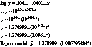
carefully recopy my work as shown below:

Important: Be sure to perform an ExpReg on your calculator to verify that the
steps above are merely a roundabout way of achieving the same result. Why do
we make you do this, if ExpReg is faster? Think of an answer (for class
discussion).
(g) Remember, 1997 is coded as 17. Begin your work by showing  , and remember to give your answer using correct units. , and remember to give your answer using correct units.
(h) Speculation is acceptable. See if you remember any history from the
1990s.
(i) Self-explanatory.
(j) Write down the source you used (printed or on-line sources are
acceptable).
|
|
|
F 10/6/06
|
No
school.
|
|
|
M 10/9/06
|
No
school.
|
|
|
T 10/10/06
|
HW due:
1. Last Thursday’s assignment (problem #4.2) will be graded. I know I had asked
you to send me an e-mail, but as of 1:11 p.m. on Saturday, 10/7, a grand
total of 0 people had sent e-mail, so let’s forget the e-mail idea. Just have
#4.2 ready for spot-check or collection today.
2. Think about an exploratory data analysis project you might be interested
in conducting. There is no need to write your idea down just yet. See the
hint below for help.
3. Read pp. 190-195 (optional) and pp. 206-214 (required).
4. Write #3.52 on pp. 168-170 and #4.4 on p. 196. See the hints below for help.
Hint for exploratory data analysis
concept:
Try to think of something that would be fun
and educational. Don’t worry too
much about practicality for the moment. If your idea is impractical (or
unethical, or whatever), I will let you know.
Hints for #3.52 and #4.4:
3.52: Try to match the graphs with their equations without using your
graphing calculator. (They are quite easy with a graphing calculator. The
best educational benefit comes from trying to perform the matching without
using a calculator.)
4.4(a) Hint: Remember that a
height-weight plot must pass through the origin.
(b) Either choice can be defended. However, if you
read ahead to part (e), you can deduce from the wording of the question that
you will be using your model to predict weight. Does that give you a clue?
(c) If you have height in L1 and weight in
L2, the transformation consists of doing log(L1)®L3 and log(L2)®L4, then STAT CALC 8 L3,L4,Y1.
The rationale is that if you are hypothesizing a power relationship where y » axb,
then by properties of logs, we have log y
» log a + b log x. (There is a
reason that precalculus is a prerequisite for this class. If you do not
remember why this equation is true, please contact me or one of the other
math teachers ASAP for a quick review of logarithms.) At any rate, from the
equation log y » log a + b log x, it should be clear that log y (namely, L4) is approximately a linear function of
log x (namely, L3). Do
you see why? If you do, then perform STAT CALC 8 L3,L4,Y1
to find the values of a and b that accomplish this linear fit.
(d) Self-explanatory. Remember, however, that your
RESID list holds differences between actual log y and predicted log y,
not differences between actual y
and predicted y.
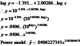
(e) As in last week’s assignment, please perform the
first part of this requirement by copying my work below. Then answer the
questions for 70 and 84 inches in the standard way. Important: Be sure to
verify that your power model matches the value you could have obtained more
quickly by punching STAT CALC A L1,L2,Y1 for
PwrReg.

Again I ask the question: Why am I making you do the inverse transform
if the calculator has a built-in power regression capability that finds the
answer so much more quickly? Trust me, there is a reason. What could it be?
|
|
|
W 10/11/06
|
HW due:
1. Read about the LSRL Top Ten.
2. Answer the following review problems: p. 207 #4.19, pp. 214-215 #4.26,
4.28.
3. Carefully read over the group selection
methodology and find the missing step(s). Write out your answer and
number it appropriately.
Note: Because today is a review
day, we will not have time for the Post
reading quiz. Instead, that will be included on tomorrow’s test.
|
|
|
Th 10/12/06
|
Test through p. 215 in text.
Please note, although there will be fewer questions this time from Chapters 1
and 2 (exploratory data analysis and univariate statistics), you cannot
forget any of what you learned there. For example, notational questions
similar to those that so many people had trouble with on Test #1 may make a reappearance. Chebyshev’s Theorem, which did not make the cut
last time, will probably appear this time.
The topics emphasized most heavily today will be regression, curve fitting, inverse transformation, residual plots,
scatterplots, cause and effect, and interpretation
of regression. Be sure to reread the LSRL Top Ten list.
|
|
|
F 10/13/06
|
HW due: Read pp. 215-226.
|
|
|
M 10/16/06
|
No
additional HW due. Use this weekend to patch up any gaps in your previous
assignments.
In class: Groups will meet and will write up a project concept. The report
will be due on Wednesday, 10/25.
Group 1: Sam (leader), Denny, Matt
Group 2: Michael R., Alex, Oliver
Group 3: In-Sung, Julian, Rick
Group 4: Nicholas, Kellie, Peter (note change: Kellie will be a
project leader next quarter)
Group 5: Michael W., James, Marcus
Other notes: Graphical depiction of Simpson’s Paradox.
|
|
|
T 10/17/06
|
HW due: Each group should produce a proposal of approximately
half a page. State your research
question very clearly at the outset, in the form of a question
(obviously). Describe the outline of what you will do. Estimate the length of
your final report, estimate the day on which you will be showing a rough
draft (preferably Oct. 23 or 24), and if possible, indicate approximately how
the workload will be divided among the group members. The last portion is
optional for the moment, but you might as well think about it now. If your
group leader is absent today, he must deputize someone else to deliver the
proposal. Use standard HW format or a computer printout (your choice).
|
|
|
W 10/18/06
|
HW due: Short progress report (will be conducted orally).
In class: Finish all textbook material through p. 226, including Simpson’s
Paradox. The remainder of the time was supposed to be available for group
work, but we will have to do that tomorrow.
|
|
|
Th 10/19/06
|
HW due: Read this article
concerning lurking variables. Be prepared for a Short Quiz (10 pts.) on the reading and lurking variables in
general.
In class: Following the quiz, the entire period is devoted to group work.
This would be a good opportunity for you to show me your consent form, data collection instrument (i.e., survey), and raw data
table format. That way, any bugs or missteps can be caught early, before
they adversely affect the execution of your project. If you already have
collected some data, bring them in so that we can discuss them, but that is
not assumed.
|
|
|
F 10/20/06
|
No
class today (Form VI retreat).
|
|
|
M 10/23/06
|
No
additional HW due. However, each project leader should plan to give an oral
report on project-related accomplishments. If the project leader will be
absent, he must deputize someone to fill this role.
Notice: If your project is running
behind schedule, today is the last day on which you can apply for a 48-hour
extension. An extension may be granted if the situation warrants, but
approval is not automatic and should not be assumed. Extension requests must
be made in writing.
In class: Responder system questions on LSRL, r, and r2.
|
|
|
T 10/24/06
|
Last day for 24-hour extension
requests. An extension may be granted
if the situation warrants, but approval is not automatic and should not be
assumed. Extension requests must be made in writing.
In class: Group work.
|
|
|
W 10/25/06
|
Project first draft due today
(including group leader report).
Please read the first draft guidelines
carefully. Because the quarter ends Friday, extensions cannot be granted
without special permission, and the maximum length of an extension will be 48
hours. However, no 48-hour extension requests will be considered after
Monday, and no 24-hour extension requests will be considered after Tuesday.
Rationale: If you are fewer than n
hours from a deadline when you realize you will be at least n hours late, then it is obvious that
you have not assessed your intermediate progress correctly.
|
|
|
Th 10/26/06
|
HW due:
1. Consider carefully whether it would be best to run our full-class project
as a census, a simple random sample (SRS), or a stratified random sample. Write your recommendation and 2-5 sentences
of justification. Your answer need not match the anonymous answer you
submitted yesterday. There is no “right” or “wrong” answer to this question.
The points will be awarded based on the quality of the arguments you give.
Reminder: If, at any time during
the course, you find a term that is unclear to you, you should feel free to
look it up in your textbook’s index or in the glossary found under the Essential Links section of the Statistics
Zone.
2. Write a paragraph in which you describe how you would design the
methodology of the study. You need not justify your choice here; simply
describe what you think makes sense. For example, would you use face-to-face
polling, focus groups with one-way mirrors, focus groups with note-taker(s)
present in the room, written surveys distributed by U.S. mail, written
surveys distributed in person but gathered from drop boxes, Web-page surveys
(similar to quantescape.com/neptune),
written or Web-posted surveys with data received by text messaging, or
something else? Would you gather quantitative data, categorical data,
qualitative responses, or some mixture of these? There are literally dozens
of variations you could consider. Describe how you would ensure that the data
were meaningful, credible, and useful, and how you would protect the identity
of the subjects.
|
|
|
F 10/27/06
|
HW due: For the proposed
survey questions that were distributed in class yesterday, find one good
thing to say about each one, as well as one criticism of each one. Do all of
them, even the ones that were discussed in class. Have your answers written
out so that you can instantly respond if called upon.
|
|
|
M 10/30/06
|
No
additional HW due. Please take a well-deserved break to celebrate all 5
groups’ having turned in their projects last week.
|
|
|
T 10/31/06
|
HW due: Now that you know quite a bit more about how to
write questions, carefully write 5 questions for our class survey. Try to
cover several aspects of the subject. If you wish to write more than 5
questions, that is fine.
|
|


