|
M 11/3/14
D
|
HW due (both periods):
1. Rewrite your solutions from Friday so that they are neat, complete,
correct, and informative. Answers should be circled, and your writeup should probably use several complete English
sentences so that the interpretation does not require an advanced degree in
mindreading. No cryptic writeups, in other words!
Explain yourself.
It counts as an explanation only if it
makes sense to a reader who has not already done the same or similar work.
Note: Time spent on this task does
not count toward your time log, if any, since you were supposed to have done
it last week.
2. Read pp. 313-320, 323-331 (middle). You may omit the Bayes’
Rule box, since it is not an AP topic. More advanced students will want to
read it anyway.
3. Write #6.36 on pp. 311-312.
4. Write #6.42, 6.44, 6.48, and 6.50 on pp. 320-321.
5. Write #6.66abcdefghijkl on pp. 333-334.
|
|
|
T 11/4/14
E
|
HW due (both periods):
1. Read pp. 335-343 (reading notes required, as always).
2. Read Activities 6.2 and 6.3 on pp. 347-348. Choose one of them and write
up a simulation plan that will utilize a
table of random digits. You are not required to execute the plan; simply
write up the steps of your plan and how you intend to estimate the
parameter(s) of interest.
|
|
|
W 11/5/14
F
|
No class.
|
|
|
Th
11/6/14
G
|
HW due (both periods):
1. Read pp. 357-365.
2. Classify each of the following as not
a random variable, discrete random variable, or continuous random variable. You may abbreviate the term “random
variable” as r.v.
(a) pi
(b) the length of time, to the nearest second, that the murmuring lasts after
head prefect Jim Hurson rings the announcement bell and says, “Please settle
down”
(c) the diameter of an egg splat when a failed egg is dropped from the roof
of Marriott Hall to the concrete below
(d) the number of students who show up for a special announcement in the
Little Sanctuary
(e) the number of students who have a doctor’s appointment and therefore miss
lunch
(f) the number of heads in a set of 35 random coin flips of a fair coin
(g) the number of heads in a set of 35 random coin flips of an unfair coin
|
|
|
F 11/7/14
|
No school.
|
|
|
M 11/10/14
A
|
HW due (both periods):
1. Read pp. 367-383. Reading notes are required, as always.
2. Write #7.20 on p. 371, #7.26 on p. 372, #7.28 on p. 383, and #7.41 on p.
385.
3. Current or former calculus students only: Briefly explain the connection
between continuous random variables and the calculus.
|
|
|
T 11/11/14
B
|
Period 3 HW due: Read pp.
386-394; write #7.42 and 7.44 on pp. 385-386.
Period 4: No class.
|
|
|
W 11/12/14
C
|
Period 3: No class.
Period 4 HW due: Read pp. 386-394; write #7.42 and 7.44 on pp. 385-386.
|
|
|
Th
11/13/14
D
|
HW due (both periods):
1. Read pp. 397-412.
2. Write #7.64abcdef. Important: Do
each problem by using the table at the end of your book, and then use your calculator
(normalcdf) to check your answer. The first one is
done for you as an example. Be sure to “X out” your normalcdf
work, since calculator notation is not permitted.
(a) P(z < 1.75) = 0.9599 by table. Check: normalcdf(-9999,1.75,0,1)
= 0.95994.
|
|
|
F 11/14/14
E
|
Period 3 HW due: Read
chapter summary on pp. 430-431, plus pp. 445-459.
Period 4 HW due: Everything above, plus you need to listen to both of the
following short NPR stories on experimental design for Ebola vaccines. There
may be a discussion and/or an open-notes quiz based on the content of the
stories.
1. Original
story (from late September or early October, before Thomas Eric Duncan
died in Texas)
2. Follow-up
story (from 11/11/2014)
|
|
|
M 11/17/14
F
|
No class.
|
|
|
T 11/18/14
G
|
HW due (both periods):
1. Read pp. 461-466. Remember that we use the notation p for what your book calls  , and we use , and we use  for what your book
calls p. In other words, we use for what your book
calls p. In other words, we use  to denote the sample
proportion (statistic) and p for
the population proportion (parameter), a.k.a. probability. to denote the sample
proportion (statistic) and p for
the population proportion (parameter), a.k.a. probability.
2. Write #7.106abcd, 7.109-7.116 all, and 7.119-7.123 all on pp. 431-433. You
will need to start this assignment at least a little bit over the weekend in
order to finish on time.
Note: Office hours for Tuesday
afternoon are canceled on account of illness.
|
|
|
W 11/19/14
A
|
HW due (both periods):
1. If you have not already done so, complete the long assignment that was due
yesterday.
2. Prepare for a “highly likely” quiz that rehashes yesterday’s pop quiz. The
Block 4 version of the quiz is provided
for your study benefit (inspired by the photo that Roy took, but now at
higher resolution). The formulas for mean and variance of a binomial r.v. (np and npq, respectively) and the formula for the variance of a
geometric r.v. (namely, q/p2) will
be provided for you. The formula for the mean of a geometric r.v., namely 1/p,
is not provided on the AP formula sheet and will not be provided for you.
3. Perform Exploration 8.2 on p. 473. (Note:
Do not read the material on p. 474, which is complicated and completely
unnecessary.) Your calculator has a randBin
function (found under the MATH PRB #7 command) that generates random outputs
from a binomial distribution. The syntax is randBin(n, p)
to generate a single random output using parameters n for number of trials and p
for the single-shot probability of success, or randBin(n, p,
m) to generate a list of m random binomial outputs of the
desired type.
Your goal in Exploration 8.2 is stated at the bottom of p. 473: to show that
the simulated results for mean and s.d. are close
to the theoretical values. You should perform this exploration for several
different values of n and p and summarize your findings in an
appropriate manner. Note that by using randBin(n, p,
m)/n and “STO”ing the result into a list,
you can generate your simulated results in a jiffy and can bypass most of the
gobbledygook printed in your textbook. For best results, make sure that you
use a value for m that is large
(several hundred or more).
Note: This exploration is not repeating what we did in Excel
yesterday, which was to model the binomial and geometric distributions.
Instead, you are modeling the sampling distribution of the sample proportion
( ). ).
|
|
|
Th
11/20/14
B
|
Period 3 HW due: Use either
Excel or your calculator to demonstrate that the mean and s.d.
of the sampling distribution of  for n = 200 are reasonably close to for n = 200 are reasonably close to  and and  respectively, respectively,
provided that the underlying distribution is either (a) a random normal
variable with mean 7 and s.d. 3.5 or (b) a
uniformly distributed continuous random variable with minimum 0 and maximum
1.
Period 4: No class.
|
|
|
F 11/21/14
C
|
Period 3: No class.
Period 4 HW due: Use either Excel or your calculator to demonstrate that the
mean and s.d. of the sampling distribution of  for n = 200 are reasonably close to for n = 200 are reasonably close to  and and  respectively, respectively,
provided that the underlying distribution is either (a) a random normal
variable with mean 7 and s.d. 3.5 or (b) a
uniformly distributed continuous random variable with minimum 0 and maximum
1.
Period 4: No class.
|
|
|
M 11/24/14
D
|
HW due (both periods):
1. Read the chapter summary on pp. 469-470.
2. Reread the top of p. 457. The “> 30 rule” referred to in the green box is
generally safe, but it is not valid in the case of extreme skewness or extreme outliers. Please make a notation to
that effect. (More on this subject can be found in a recent blog entry, but that is optional reading.)
3. Mark up (using pen or pencil, your choice) the definition at the top of p.
470, changing all occurrences of p
to  , as well as changing all occurrences of , as well as changing all occurrences of  to p. Therefore, the definition becomes a
definition for “Sampling distribution of to p. Therefore, the definition becomes a
definition for “Sampling distribution of  ” (not p), and
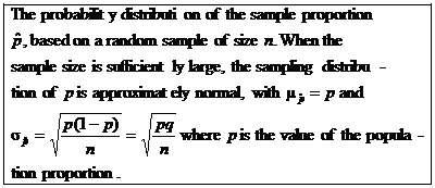
the right-hand column becomes this: ” (not p), and
the right-hand column becomes this:

4. On p. 470, write #8.32-8.37 all. The first one is done for you as an
example, but in order to earn full credit for the assignment, you must either
copy it onto your homework paper or improve upon the presentation below.
8.32. Let X = nicotine content (in
mg) of a randomly chosen cigarette.
Given: 
We are not
given that X is a normally
distributed r.v., but the CLT [p. 455] guarantees
that the sampling distribution of  is approx. is approx. 
Reason: n
> 30, and manufacturing processes in the real world do not exhibit extreme
skewness. Outliers, if any, would be rare.
Thus P( < 0.79) = 0.159
by calc., and P( < 0.79) = 0.159
by calc., and P( < 0.77) = 0.00135
by calc. < 0.77) = 0.00135
by calc.
normalcdf(–999,.79,.8,.01)
ENTER, normalcdf(–999,.77,.8,.01) ENTER
In class: Guest speaker, Mr. Joe
Morris, STA ’62. Mr. Morris will speak for approximately half the period
on the subject of statistical models for technology growth.
|
|
|
T 11/25/14
E
|
HW due (both periods): Send
yesterday’s HW scan by hitting “Reply” to the e-mail that arrives in your
inbox. There is no additional written HW due.
|
|
