|
Th
3/1/012
|
HW due: Read pp. 562-564, 573M-574; write Activity
10.2 on p. 575, plus #10.73 (following the PHASTPC steps from yesterday’s
handout), #10.95.
|
|
|
F 3/2/012
|
HW due: Read the material below; write #10.76.
P-value = P(a result as extreme as or more extreme than this one will be
obtained in the future | H0
true)
P(Type I error) =  = P(rejecting H0 | H0
true) = P(rejecting H0 | H0
true)
P(Type II error) =  = P(failing to reject H0 | H0 is false in some particular way) = P(failing to reject H0 | H0 is false in some particular way)
The purpose of is to serve as a
cutoff for P-values. If P < , we say that we have achieved significance at the = [whatever] level,
and we have found evidence for the alternative hypothesis. On the other hand,
if P > , we say that we have failed to find evidence for the
alternative hypothesis. But note! When we set a significance level of , then by definition, chance alone will give us a result
significant at that level a certain percentage of the time. If = 0.05, for example,
then by definition, 5% of the experiments that we run will have P-values below 0.05 even if there is no real experimental
effect at all. That’s fine if we call the hypothesis in advance (remember
the legend of Babe Ruth and the “called shot”), but it is not OK if we go dredging through data
looking for the occasional result that has a P-value below 0.05.
|
|
|
M 3/5/012
|
HW due: Write #10.85 with the full PHA(S)TPC
steps.
|
|
|
study guide
|
The full solution to #10.85 is below. Match your
work against this, and make corrections as needed. Work may be collected on
or after Wednesday, 3/7.
Solution:
Let p = true proportion of cars purchased
in the “certain metropolitan area” that are white
H0: 
Ha: 
Assumptions for 1-prop. z
test:
Is  ? Yes, since in a large metro area, 10n = 10(400) = 4000 is surely a lower bound for car sales in any
period of longer than a few weeks. ? Yes, since in a large metro area, 10n = 10(400) = 4000 is surely a lower bound for car sales in any
period of longer than a few weeks. 
SRS? “Random” was stated; assume close enough to SRS to
proceed.
Is  ?
Yes, since ?
Yes, since 
Is  ? Yes, since ? Yes, since 
Test statistic: z = 
P-value = 0.0124
Conclusion: There is good evidence at the = 0.05 level (but
not at the = 0.01 level) that the
true proportion of cars purchased in this metro area that are white is not
equal to 20%.
|
|
|
T 3/6/012
|
Test (100
pts.) on Chapters 9 and 10. The
optional portions of §10.5 (pp. 564-570) will not be included. However, you
do need to know the conditional-probability definitions of Type I and Type II
error listed in the 3/2 calendar entry.
|
|
|
W 3/7/012
|
HW due: Read pp. 583-595, being sure to ignore the df formula on p. 586, p. 587, p. 588 (in paragraph 8), p.
590 (in paragraph 8), and p. 593 (in paragraph 8). We will never use that
formula! Nowadays, we let the calculator or computer software figure it out for us.
|
|
|
Th
3/8/012
|
HW due: Read pp. 595-597, 606-614.
|
|
|
F 3/9/012
|
HW due: Write #11.29, 11.35. For #11.35, use a full PHA(S)TPC procedure for part (c).
In class: Guest speaker from the NRC, Ms. Suzanne Schroer. Ms. Schroer is a
nuclear engineer and a graduate of the University of Missouri at Rolla.
Please bring some good questions for her!
|
|
|
M 3/12/012
|
Mr. Kelley will be your substitute teacher today.
There is no additional HW due, but your in-class
assignment is to develop (A) a draft proposal for an experiment, (B) a draft
list of project milestones with dates, and (C) a preliminary estimate of the
power that your test (using = 0.05) would have
against the ES you realistically expect to see.
Requirements to keep in mind as you prepare these 3 responses are as follows:
1. Your study must be an experiment.
2. A 2-sample t test, not a
1-sample t test on paired
differences, should be the appropriate test to use. You will be measuring
means, not proportions.
3. You will need at least 20 data points in each of 2 groups. That means a
total of at least 40 experimental units or 40 test subjects, since this is a
2-sample experiment. If your estimate in part (C) reveals low power (70% or
80% is a good target), you should look at using a larger sample size and
re-running your power calculations.
4. In order to answer part (C), you will need to begin by estimating the s.d. for each of your samples. Note: Since you have not gathered any data yet, these estimates
must either be “picked out of the blue sky,” based on a small pilot study, or
constructed using some common-sense estimation techniques. Then, you must
estimate the s.e. of the statistic  by using the formula by using the formula  ,
which comes from your AP formula sheet. ,
which comes from your AP formula sheet.
From the latter, you can then sketch curves for both the H0 sampling distribution and an
“Ha sampling
distribution.” Remember, the first curve would be centered on 0, whereas the
second curve would be centered on whatever you believe would be a likely ES.
Draw a thick bar (or 2 thick bars if you are doing a 2-tailed test) on your H0 curve, and clearly label
the “reject H0” and “do
not reject H0” zones. Now
read carefully: The estimated amount of the Ha curve that bleeds into the “do not reject” zone
tells you  the probability of
Type II error, and from that, you can easily compute power. the probability of
Type II error, and from that, you can easily compute power.
Exact numbers are not expected! Exact numbers are difficult to calculate. The
position of the thick bars between zones, the df
for the test, and the probabilities (areas under the curves) all depend on the sample sizes as well
as the s.d. estimates, neither of which may be
known accurately before the test is run. Not only that, but the 2-sample df is difficult to compute by hand, and the formula is so vicious that it is not even included on the AP
formula sheet.
Group assignments for this project (“An Experiment With 2-Sample t Tests”) are as follows:
Group 1: Sam (leader), Karl, Miles
Group 2: Nathan (leader), Matt, Kieran
Group 3: Frederik
(leader), Steven, Joe, Bogdan
|
|
|
T 3/13/012
|
HW due: Parts (A), (B), and (C) from yesterday’s
in-class assignment. If the group leader is absent today for any reason, he
should designate a deputy to submit the assignment. If nobody submits the
assignment, all group members will earn a zero (scored as a double HW).
|
|
|
W 3/14/012
|
HW due: Revise parts (A), (B), and (C) from
yesterday’s assignment, following the feedback given in class. The power
estimate requires some descriptive text in addition to the sketches. Be sure
to document your assumptions clearly. If you have any rationale for your
estimates, even if it is only a “gut feeling,” be sure to state how you came
up with it. Use proper notation.
|
|
|
Th
3/15/012
|
HW due: Read pp. 619-626; write #11.41, 11.43, 11.46.
Note: For #11.43ab, show your work
in calculating the m.o.e. Of course, you can (and
should) check your work with your calculator’s STAT TESTS capability. For
part (c), perform an appropriate statistical test with all PHA(S)TPC steps. Note that #11.46 also requires PHA(S)TPC.
|
|
|
F 3/16/012
|
HW due:
1. Continue working on your group project. Each project leader (or an
appointed deputy, if the leader is absent) will give a quick oral status
update during class.
2. Read pp. 629-632 and the summary on pp. 633-634.
3. Write Activity 11.3 on p. 633.
4. Write #11.64 on p. 635. Note:
This question is short-answer. PHA(S)TPC steps are
not required. Whew!
|
|
|
M 3/19/012
|
HW due: In honor of Stub Week and your projects that
are in progress, there is only a skimpy assignment for this weekend. Here it
is:
1. If you have not already done so, write Activity 11.3 on p. 633.
2. Read pp. 647-656.
|
|
|
T 3/20/012
|
HW due:
1. Read the solution of #12.13 that is posted below.
2. Write #12.10, showing all PHA(S)TPC steps.
3. Continue working on your project.
Solution to #12.13:
Let p1 = true
probability of phenotype 1 (tall cut-leaf)
p2
= " " " " 2
(tall potato-leaf)
p3
= " " " " 3
(dwarf cut-leaf)
p4
= " " " " 4
(dwarf potato-leaf)
H0: 
Ha: Not all
probabilities are as stated in H0.
Assumptions for  g.o.f.
test: g.o.f.
test:
SRS? Not stated; must assume in order to proceed.
Data recorded as counts?
All expected counts  1? Smallest expected count is 1? Smallest expected count is 
No more than 20% of expected counts < 5? All exp. counts
> 100 from above.
Expected counts (n = 1611) are
906.1875, 302.0625, 302.0625, and 100.6875, respectively.
Test statistic:
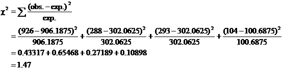
P-value = 0.69 by calc. [The
keystrokes are 2nd DISTR 7 1.47,99999,3 ENTER. However, you cannot write
that.]
Conclusion: There is no evidence (n
= 1611, = 1.47, df = 3, P =
0.69) that the true proportions of the 4 phenotypes differ from those
predicted by Mendel’s laws of genetics.
|
|
|
W 3/21/012
|
HW due: Start reading the book How to Lie With Statistics. There will be a discussion and a quiz
after we return from spring break. Reading notes are required, as always.
|
|
|
|
Spring break, March 22–April 1.
|
|