STAtistics / Mr. Hansen 12/15/2010

Name: ___________KEY___________ Bonus (for Mr. Hansen’s use only): ________

Test through Chapter 8 (Calculator Required)

Rules	You may not write calculator notation anywhere unless you cross it out. For example, terms like binompdf and normalcdf may result in small point penalties. Use diagrams and/or formulas to justify your answers instead. Adequate justification is required for free-response questions. All final answers in free-response portions should be circled or boxed. Decimal approximations must be correct to at least 3 places after the decimal point, and preferably should contain at least 3 significant digits.
Part I	Notation and Definitions.
1.	Chapter 8 is all about ___sampling____ distributions, and we considered two specific examples: (1) the ___sampling____ distribution of ____ (symbol), the ____sample_____  _____mean______ , and (2) the ___sampling____ distribution of __ (symbol), the ____sample_____  ___proportion__ .
2.	Any __statistic____ (median, range, IQR, etc.) can have a ___sampling____ distribution. However, the AP Statistics syllabus considers only a few of the most common ones. One requirement is that a ___sampling____ distribution must have a fixed value for _n__ (symbol), the sample size.
3.	The difference between and is that the former is the s.d. of _a quantitative variable*_ , while the second is the s.d. of [explain briefly below] the sample means (plural) from all possible samples of a certain size from the same population. * Also acceptable for first blank: “a population,” “some variable of interest,” “x,” or “data”
4.	Any binomial distribution in which p > 0.5 is symmetric   skew right   skew left [circle one].
5.	State the CLT.
	If then the sampling distribution of approaches as .
6.	CLT stands for ___Central__  ____Limit___  __Theorem____ .
7.	Explain briefly why, in cases where it is not possible to put an upper bound on , the improper use of CLT could have disastrous multi-trillion-dollar consequences.
	If an investor makes investment decisions or risk-analysis decisions based on Gaussian (normal) models that depend upon the CLT, then he or she could severely miscalculate the likelihood of a catastrophic meltdown of a sector of the economy or (in the case of the Crash of 2008) the entire economy. The future is not nearly as predictable as the believers in the CLT think it is. Some quantities, such as the s.d. of AIG’s bets on the subprime mortgage market, cannot have any reasonable upper bounds attached to them because of dependencies and ramifications in other parts of the economy.

Part II	Computation.
8.	Explain why, in the real world, we would never know the true value of p for a political poll in which p is the proportion of support for a candidate among the likely voters.
	The true proportion, p, is a parameter. In the real world, we are not able to know the values of parameters. The whole purpose of our course is “using statistics to estimate parameters.”
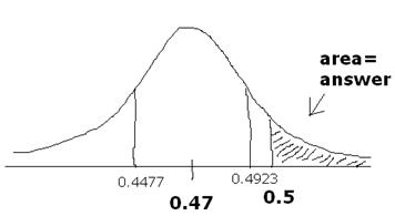
9.	Assume, contrary to reality, that p = 0.47 for the situation described in #8. If 500 likely voters are randomly polled, make a sketch to estimate the probability that the poll shows more than 50% support for the candidate, even though p is truly less than that. Mark values along your x-axis.
	Since the sampling distribution of is approximately normal (see #10), we can find the probability that if we consider the mean, namely 0.47, and the s.d., which is given by or about 2.23 percentage points. The shaded area to the right of 0.5 appears to be about 0.1. [The “correct” answer is 0.0895, but you were not required to come up with that. On Thursday’s test, however, you may be required to perform the computation, using either your calculator or the z table.]
10.	Prove, by checking and verifying the rules of thumb, that your method in #9 is valid.
	1. Is N at least 10n? Assume there are at least 5000 likely voters, and then we have it.
	2. Is np at least 10? Yes, 500(0.47) = 235 > 10.
	3. Is nq at least 10? Yes, 500(0.53) = 265 > 10.
	Therefore, the normal approximation is valid here as a substitute for the binomial distribution. [The “correct” distribution is binomial, but it is awkward to work with, especially for large values of n.]

11.	Mr. Hansen’s true mean systolic blood pressure is 135, with a standard deviation of 10 points. In a series of 50 readings, made at random times of the day over a period of time, estimate the probability that the sample mean is below 133. Make a reasonably accurate sketch, and mark appropriate values on the x-axis. Show all relevant work.
	The sampling distribution of is closely approximated by a normal distribution having mean 135 and s.d. given by The sketch looks almost exactly like the sketch on the previous page, except that the “inflection point” tick marks will be at 133.6 and 136.4, and it is the area to the left of 133 that must be shaded. Once again, 0.1 is a reasonable estimate. The “correct” answer is 0.0786, which you should be able to compute via calculator or z table.
12.	In #11, is it necessary to assume that the population distribution of systolic blood pressure readings is normal? Why or why not?
	No, because the CLT starts to take effect for n exceeding approximately 25 or 30. Since we have n = 50 here, and since Mr. Hansen’s blood pressure (like nearly all quantities from the natural world) fluctuates within a band having no severe outliers, we can apply the normal approximation for probabilities concerning even though the population data distribution may not be normal.