AP Statistics / Mr. Hansen
Answer Key for Big Quiz #1 (10/12/2000, rev. 10/20/2004)

Name: ____________________

1.

weak negative linear
explanatory
response
10.1124%

2.

linear correlation coefficient [all 3 words required]
coefficient of determination

3.

the difference is too large to be plausibly explained by chance

4.

yhat = a + bx in TI-83 notation; yhat = b₀ + b₁x in AP notation
a = intercept (b₀ in the AP notation)
b = slope (b₁ in the AP notation)
r (s_y / s_x)
sometimes [truly meaningful only if x can realistically have values near 0]
a = ybar – b(xbar); shown on AP formula sheet as b₀ = ybar – b₁(xbar)

5.

zero

6.

SSE (sum of squared residuals)

7.

y – yhat, i.e., the difference between actual y and value predicted by model

8.

11
(2.5, 131.6), since it is a LSRL property that (xbar, ybar) is always on the LSRL
(0, 0) must be on the scatterplot, though not necessarily on the LSRL
No. Joe’s predicted location at time 2.5 hours is 131.6 miles, but there is no guarantee that he will be exactly at that distance. [If the linear fit is good, he should probably be fairly close to that distance.]

9.

none

10.

a data point with a large |residual|
a data point that has a large effect on the LSRL

11.
(a)

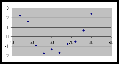
Although there is a strong positive linear correlation (r = 0.970) between X values and Y values, the residual plot shows a pattern suggesting that the linear fit is not appropriate:

(b)

yhat = a + bx
yhat = -13.91569091 + 0.525677273(56.5)
yhat = 15.785

(c)

linear fit between x and log y yields a = 0.495316683, b = 0.012139633
log yhat = a + bx
10^{log yhat} = 10^a + bx
yhat = (10^a) (10^bx)
yhat = (10^a) (10^b)^x
Answer: yhat = 3.128359703 (1.028346877)^x, which has the required form. [Note that a and b in the required form are different from the a and b in the linear regression.]

(d)

ExpReg gives same values: yhat = ab^x, where a = 3.128359703, b = 1.028346877.

(e)

Using yhat = ab^x = 3.128359703 (1.028346877)^x from (c), we have
yhat = 3.128359703 (1.028346877)^56.5 = 15.178

(f)

Since the X values are equally spaced, we can look at ratios between successive Y values:

1.127063139
0.96823183
1.101872599
1.183963977
1.107900871
1.166823542
1.112223593
1.139681727
1.143712799

These values are close enough to suggest an approximately constant ratio, which is the hallmark of an exponential model.

However, the residual plot is still not very random:



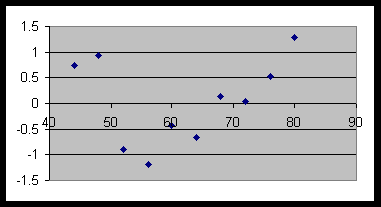
Although the pattern is less pronounced than before, there is still a lack of randomness. [Neither exponential nor power regression gives a very good fit. However, both give a lower SSE than the original linear fit, which is certainly a good thing. How would we calculate SSE, by the way? See below for answer.]












How to calculate SSE efficiently on your calculator:

Perform 1-Var Stats on your residuals (called RESID if you are using a built-in regression). Unfortunately, although it would seem logical that you could punch in STAT CALC 1-Var Stats 2nd LIST RESID ENTER, the word "RESID" is a reserved word and cannot be used for 1-Var Stats. However, you can "STO" the RESID list into a new list called, say, R4, and then punch in STAT CALC 1-Var Stats 2nd LIST R4 ENTER. The SSE would be shown as S x², which of course, should never be confused with (S x)².

What if you are using a "custom" regression where you have to calculate residuals manually? Suppose that your residuals are stored in L₅. Then you would punch STAT CALC 1-Var Stats L₅ ENTER. As before, you would read the SSE as S x².