scatterplot
residual
pattern, or residuals whose absolute values show a trend for extreme values of X
log(Y)
exponential growth
proportional to the amount present [see note below]
ratio
exponential
Note on detection of exponential growth
The notion of rate of change being proportional to the amount present is a "calculus-style" definition of exponential growth. A more "precalculus-style" definition is to have the Y value increasing at a constant percentage rate, i.e., by a constant multiple for any step change in X. A population, a bacterial colony, or a bank account that are growing at a 2% annual rate would all be examples of exponential growth, since the multiplier (1.02) is constant for any 1-year change in X.
STAT CALC 0 (ExpReg)
log(Y)
STAT CALC 8 L1,L3
log(yhat)
"f " [which in this case is the antilog function, a.k.a. "10 to the"]
10log(yhat) = 10a + bx
yhat = ABx [after some precal-style simplifications]
STAT CALC 0 (ExpReg)
residual
origin
power function fit
proportional
log(X)
log(Y)
STAT CALC 8 L3,L4 [see note below]
r
residual
Note on checking linear relationship between log(X) and log(Y)
Instead of using L3 and L4, you could create lists LOGX and LOGY and test them as follows, where ®
denotes the "STO" key on your TI-83:
log(LXLIST)®
LOGX
log(LYLIST)®
LOGY
STAT CALC 8 LLOGX, LLOGY
STAT CALC A (PwrReg)
log(X)
log(Y)
STAT CALC 8 L3,L4
log(yhat)
"f " [which in this case is the antilog function, a.k.a. "10 to the"]
10log(yhat) = 10a + b log x
yhat = AxB
STAT CALC A (PwrReg)
residual
quadratic, cubic, natural log, logistic, sinusoidal, etc.
r or R
residual
more small residuals than there are large residuals, but otherwise no pattern
7.
manual inversion
f –1 -ing
f -ed
f –1 (Y)
invNorm(Y), log(Y), or whatever [i.e., the purported inverse applied to Y list]
linear
STAT CALC 8 L1,L3
r
residual
f –1 (yhat) = a + bx
"f "
yhat = f (a + bx)
Nuts and Bolts for #7
f –1 (x) = 10x – 5 + 7
[Note: Here, x does not mean a value of the explanatory variable (X column). The x in the definition of f –1 is merely a dummy variable meant to illustrate the action of the function. We could just as well have said f –1 (Q) = 10Q – 5 + 7, except that the use of x is standard throughout mathematics. Besides, if you survived precal, you should be comfortable with the use of x as a dummy variable. When we perform the inverse operation, we will actually be applying f –1 to the Y column, not the X column.]
Work (required) to compute the inverse:
In f itself, y = log (x – 7) + 5.
\ In f –1, x = log (y – 7) + 5. Solve for y to get...
x – 5 = log (y – 7)
10x – 5 = 10log (y – 7)
10x – 5 = y – 7
10x – 5 + 7 = y = f –1(x)
Punch in col. 3 (say, L3) as 10^(L2–5)+7 ENTER. [This is calculator notation, meant for your benefit, never to be used on tests unless you cross it out.]
Punch STAT CALC 8 L1,L3 ENTER to do a linear fit between cols. 1 and 3.
The LSRL gives you –4.31336637 + 1.072296107x as a way of taking an input (x in col. 1) to produce an output (in col. 3). That is, col. 3 = –4.31336637 + 1.072296107 (col. 1), or to put this in math notation, the eqn.
f –1 (yhat) = –4.31336637 + 1.072296107x summarizes the relationship between cols. 1 and 3.
Apply f to both sides:
f (f –1 (yhat)) = f (–4.31336637 + 1.072296107x)
But on the LHS, f of f –1of anything is just the thing itself. On the RHS, remember that f (Q) = log (Q – 7) + 5 because of how f was given to us at the very beginning. In other words, f takes its input, subtracts 7, takes the log of the result, and then adds 5. When we perform f on the rather messy expression –4.31336637 + 1.072296107x, we get log (–4.31336637 + 1.072296107x – 7) + 5 on the RHS. When you simplify LHS and RHS, which you should be able to do in your head, you get
yhat = log (–11.31336637 + 1.072296107x) + 5
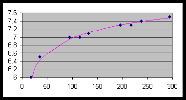
Store this eqn. into Y1 so that you can create a scatterplot. Here are the keystrokes in case you need step-by-step instructions:
Press Y= key, then define Y1 as log(VARS 5 EQ 2 + VARS 5 EQ 3 X–7)+5.
Define a scatterplot with Xlist=L1, Ylist=L2. See how closely the curve fits the data!
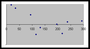
Are we finished? No, since we need to check the residual plot. Unfortunately, since we didn’t use a "built-in" regression, we must compute the residuals manually. Recalling that residuals are defined to be y – yhat, we punch in a 4th col. defined as L2–Y1(L1) and build a scatterplot involving L1 and L4, i.e., a residual plot. Because this residual plot (see below) appears to show no pattern, we say that the model
yhat = log (–11.31336637 + 1.072296107x) + 5
is an acceptable fit to the data. The model predicts y = 7.175 when x = 150 (see work below).
yhat = log (a + bx – 7) + 5
yhat = log (–11.313... + 1.072...(150) ) + 5
yhat = 7.175
Residual plot: